
Table of Contents
General terms and explanations
Databricks – multi-cloud Lakehouse Platform based on Apache Spark.
Multi-cloud Lakehouse Platform
A multi-cloud Lakehouse Platform is a data architecture that combines data lake and data warehouse features and runs across multiple cloud providers (like AWS, Azure, and Google Cloud). It allows organizations to store and analyze data seamlessly across clouds, avoiding vendor lock-in and improving resilience and flexibility.
Example:
A company uses Databricks on AWS for data science and on Azure for business analytics, all within the same Lakehouse framework.
Lakehouse Platform
A Lakehouse Platform is a modern data architecture that combines the features of data lakes and data warehouses. It allows organizations to store large volumes of raw data (like a data lake) while also supporting structured data management, transactions, and performance optimizations (like a data warehouse). This unified approach simplifies data workflows and supports both analytics and machine learning.
Data Lake
A Data Lake is a centralized repository that stores all types of data—structured, semi-structured, and unstructured—at any scale, in its raw format. It’s ideal for big data, machine learning, and flexible analytics use cases.
Data Lake – Example
A company collects logs from its website, images from users, and raw sensor data from IoT devices. All this diverse, unstructured data is stored in a data lake like Amazon S3 or Azure Data Lake Storage, where it can later be cleaned, processed, and analyzed.
Data Warehouse
A Data Warehouse is a structured system optimized for querying and reporting. It stores cleaned and processed data in a predefined schema, typically used for business intelligence and analytics.
Data Warehouse – Example
The same company processes its sales, customer, and product data into clean tables and loads them into a data warehouse like Snowflake, Google BigQuery, or Amazon Redshift. This is then used by analysts to create dashboards and run business reports. SQL (Structured Query Language) is most commonly associated with Data Warehouses, because:
- SQL is used to query, aggregate, and report on that data efficiently.
- Data warehouses store structured data in predefined tables.
Apache Spark
Apache Spark is an open-source distributed computing engine designed for big data processing. It allows you to process large datasets in parallel across multiple machines, using languages like Scala, Python, Java, or SQL. Spark supports batch processing, streaming, machine learning, and graph analytics — all in one unified platform.
Apache Spark – Example:
A company uses Spark to analyze petabytes of clickstream data from their website in real time and also train machine learning models on historical user behavior.
Computing Engine
A computing engine is a software framework or system that processes data and performs computations. It manages tasks like data transformation, analysis, and parallel execution across CPUs or clusters. Examples include Apache Spark, Apache Flink, and TensorFlow.
How Databricks Works: Control Plane vs Compute Plane
Databricks separates its architecture into two main parts: the control plane and the compute plane.
- The control plane is managed entirely by Databricks. It handles backend services like the web interface, notebooks, job scheduling, and APIs. This part always runs in a Databricks-managed environment — you don’t have access to or control over its infrastructure. Metadata such as notebooks, job configs, and logs is stored here, typically in the region where your workspace is hosted.
- The compute plane is where your data is actually processed.
There are two types of compute planes:
- With serverless compute, Databricks manages the infrastructure for you. It’s a fully managed experience — similar to a SaaS model — where you don’t need to worry about provisioning or scaling resources.
- With classic compute, the compute resources run inside your own cloud account (AWS, Azure, or GCP), within your network. You have more control over infrastructure but also more responsibility for managing it.
Note: In all cloud environments, even if the Databricks workspace appears integrated into your cloud account — showing up in your cloud portal, using your cloud billing, or connecting to your IAM setup — the control plane still runs in a Databricks-managed environment. The core backend services remain outside your direct control, regardless of the cloud provider.
Understanding the Core Concepts of Databricks
Imagine your company generates a lot of data every day. To build a robust system to handle it, your teams need to understand the key components. This chapter explains the architecture of that system, adding technical details to the foundational concepts.
Step 1: Storing Your Raw Data
First, your company needs a central, scalable place to keep all its raw information.
The Data Lake
Your company’s Data Lake is built on top of cloud object storage (like AWS S3, Azure Data Lake Storage, or Google Cloud Storage). This provides a highly durable and cost-effective foundation for storing massive volumes of data in any format.
The Databricks File System (DBFS)
To make this cloud storage easy to use, Databricks provides the Databricks File System (DBFS). This is a filesystem abstraction that allows your teams to interact with files in object storage using familiar directory and file commands, as if they were on a local machine.
An Example
Your company’s IoT devices generate thousands of JSON files daily. These are landed in an S3 bucket. An engineer can then use DBFS to explore these files with a simple path like /mnt/iot-data/raw/ without needing to write complex cloud API calls.
Step 2: Adding Reliability and Structure
Raw data in object storage lacks the reliability of a traditional database. The next step is to build a transactional layer on top.
Delta Lake
Delta Lake is the open-source storage framework that brings reliability to your data lake. It does this primarily through a transaction log (a folder named _delta_log) that lives alongside your data files. This log is the single source of truth, recording every operation as an atomic commit and enabling key database-like features.
Delta Tables
When your company creates a Delta Table, it is creating a set of data files (in the efficient Parquet format) and its corresponding transaction log. This structure enables powerful features like:
- ACID Transactions: Guarantees that operations either complete fully or not at all.
- Schema Enforcement: Prevents bad data that doesn’t match the table’s schema from being written.
- Time Travel (Data Versioning): Allows querying the table as it existed at a specific point in time.
An Example
Your finance team saves transactional data to a ledger Delta Table. Schema enforcement automatically rejects any new records where the transaction_id is null, protecting data integrity. Last quarter, an error was made; using Time Travel, an analyst can query the table’s state from before the error to diagnose the issue.
Step 3: Automating Your Data Workflows
With reliable tables, your company needs an efficient way to build and manage the pipelines that populate them. Manually scheduling jobs, managing dependencies, and handling retries is complex and brittle.
Delta Live Tables (DLT) (aka Lakeflow Declarative Pipelines)
Delta Live Tables (DLT) (aka Lakeflow Declarative Pipelines) is a declarative framework for building and managing ETL/ELT pipelines. “Declarative” means your engineers define what they want the end result to be (the target tables and their logic), not how to do it. DLT automatically interprets these definitions to build a Directed Acyclic Graph (DAG) of the data flow. It then manages the pipeline’s execution, infrastructure, data quality, and error handling.
A key feature of DLT is enforcing data quality through expectations. These are rules defined by your team that can either drop invalid records, stop the pipeline, or log violations for later review.
An Example
Your data team needs to process user clickstream data. They write a single DLT notebook with a few queries:
- A query defines a
bronze_eventstable to ingest raw JSON data, handling schema inference. - A second query defines a
silver_eventstable that reads from thebronze_eventstable. It includes an expectation:CONSTRAINT valid_user_id EXPECT (user_id IS NOT NULL) ON VIOLATION DROP ROW. This automatically cleans the data. - A final query creates a
gold_daily_summarytable by aggregating data fromsilver_events.
Your team simply defines these transformations. DLT automatically understands the bronze-to-silver-to-gold dependency, schedules the jobs, and enforces the data quality rule, all without manual orchestration.
Step 4: Governing Your Entire System
As your company’s data assets grow, managing them securely becomes critical.
Unity Catalog
Unity Catalog is the centralized, fine-grained governance solution for your Databricks Lakehouse. It provides a single place to manage data access policies, audit usage, and discover assets. It handles:
- Authentication and Authorization: It controls who users are and what they are allowed to do. You can grant permissions on specific catalogs, schemas, tables, or even rows and columns.
- Data Lineage: It automatically captures and visualizes how data flows through your pipelines, from source to dashboard.
- Data Discovery: It provides a searchable catalog for all data assets.
- Auditing: It creates a detailed audit log of actions performed on data.
An Example
Using Unity Catalog, your security administrator grants the marketing_analysts group SELECT permission only on the gold_daily_summary table, ensuring they cannot access raw PII data in the bronze layer. An analyst in that group can then discover this table and view its lineage to understand its origins before using it in a report.
The Big Picture
The Lakehouse
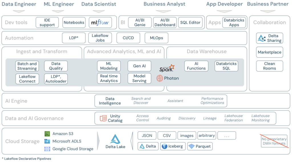
The Lakehouse is the architecture your company has built. It unifies your Data Lake and Data Warehouse, enabling both BI/SQL Analytics and AI/ML workloads on the same single copy of your data, governed by Unity Catalog.
The Data Intelligence Platform
The Data Intelligence Platform is the name for the complete Databricks product. It’s the Lakehouse architecture infused with AI to understand your data’s unique semantics, creating a more manageable and intelligent system.
System Blueprint
+-----------------------------------------+
      |        Data Intelligence Platform       |
      |   (The whole smart Databricks system)   |
      +-----------------------------------------+
                         ^
                         | (Governed By)
      +-----------------------------------------+
      |              Unity Catalog              |
      |     (Central Governance & Lineage)      |
      +-----------------------------------------+
                         ^
                         | (Pipelines Built With)
      +-----------------------------------------+
      |           Delta Live Tables             |
      |        (Declarative Pipeline Tool)      |
      +-----------------------------------------+
                         ^
                         | (Creates/Populates)
      +-----------------------------------------+
      |              Delta Tables               |
      |        (Your Reliable Data Tables)      |
      +-----------------------------------------+
                         ^
                         | (Powered By)
      +-----------------------------------------+
      |               Delta Lake                |
      |      (Reliability Layer for Storage)    |
      +-----------------------------------------+
                         ^
                         | (Sits On Top Of)
      +-----------------------------------------+
      |                 Data Lake               |
      |      (Raw Cloud Storage via DBFS)       |
+-----------------------------------------+What is DBFS and How It Fits into the Databricks Lakehouse
DBFS (Databricks File System) is a distributed file system that comes built into every Databricks workspace. It acts as a wrapper over your cloud storage (such as AWS S3 or Azure Data Lake Storage), making it easy to read and write files in Databricks using familiar file paths.
You can think of DBFS as the file interface layer of the Databricks environment.
🔧 How DBFS Works
- DBFS provides paths like
/dbfs/, which feel like local folders, but actually point to cloud object storage. - When you use
/dbfs/my-data/file.csv, behind the scenes, it interacts with your configured cloud storage (e.g.s3://...orabfss://...). - DBFS supports multiple use cases: loading raw data, saving intermediate job outputs, storing machine learning models, or staging files.
🧱 DBFS in the Lakehouse Architecture
Databricks’ Lakehouse combines the flexibility of a data lake with the performance and structure of a data warehouse. The architecture has three core layers:
- Storage Layer (the foundation):
- Built on open, low-cost cloud object storage (S3, ADLS, GCS).
- Stores all raw and transformed data (structured, semi-structured, unstructured).
- Data Management Layer (Delta Lake):
- Manages tables, transactions, schema enforcement, and versioning.
- Enables ACID operations and fast queries on data stored in the lake.
- Compute Layer (Databricks Runtime):
- Executes queries, transformations, and machine learning workflows using Apache Spark or SQL engines.
So where does DBFS fit in?
- DBFS acts as a convenient gateway to the storage layer.
- It gives users and developers a file system-like interface to interact with Delta Tables and other files — without worrying about the complexities of cloud APIs or storage paths.
- It ties the compute and storage layers together, making the experience feel unified and seamless.
💡 Summary
DBFS isn’t the lake itself, but it makes working with the lake easier. It’s a vital part of the developer and data engineering experience in the Lakehouse, enabling fast access to files and simplifying workflows across data engineering, analytics, and ML.
Core Workloads in Databricks: Analytics, Engineering, and Machine Learning
Databricks is built to support multiple data workloads on a single platform. These are the three main pillars:
1. Data Analytics
Used by analysts and business users to explore data, build dashboards, and run SQL queries.
- Tools: SQL Editor, Databricks SQL, dashboards, visualizations.
- Data is often queried from Delta Tables using SQL.
- Common use cases: reporting, KPIs, business intelligence.
2. Data Engineering
Focused on building pipelines to ingest, clean, transform, and structure raw data for analytics and ML.
- Tools: Notebooks (Python/Scala/SQL), Jobs, Delta Live Tables (DLT), workflows.
- Uses Apache Spark and Delta Lake under the hood.
- Common use cases: ETL, batch/streaming pipelines, schema enforcement.
3. Machine Learning (ML)
Used by data scientists and ML engineers to train, tune, and deploy machine learning models at scale.
- Tools: MLflow, AutoML, notebooks, experiment tracking, model registry.
- Supports libraries like scikit-learn, TensorFlow, PyTorch, and XGBoost.
- Common use cases: predictive analytics, recommendations, NLP, forecasting.
Why it matters:
All three workloads run on the same Lakehouse foundation, sharing the same data, governance, and security model — making collaboration easier and reducing infrastructure complexity.
Delta Tables
Delta Tables are a type of data table in Databricks built on Delta Lake, an open-source storage layer that brings ACID transactions, versioning, and schema enforcement to data lakes.
They allow you to read and write data just like a regular table, but with the reliability of a data warehouse and the flexibility of a data lake.
🔑 Key Features:
- ACID transactions – safe concurrent reads and writes
- Time travel – query data as it existed at a previous point in time
- Schema evolution – automatically handle changing data structures
- Efficient updates/deletes – thanks to file-level metadata and transaction logs
Example use case:
A data engineer builds a daily pipeline that loads new sales data into a Delta Table. Later, an analyst queries that table in SQL, and a data scientist uses it to train a machine learning model — all on the same consistent
Delta Lake vs Data Lake: What’s the Difference?
| Feature | Data Lake | Delta Lake |
|---|---|---|
| Storage | Raw files (CSV, JSON, Parquet, etc.) | Built on Parquet + transaction log |
| Format | No standard table format | Delta format (extension of Parquet) |
| ACID Transactions | ❌ No | ✅ Yes |
| Schema Enforcement | ❌ Weak or none | ✅ Enforced and flexible (schema evolution) |
| Data Versioning | ❌ No (unless implemented manually) | ✅ Time travel and rollback supported |
| Performance | Basic (depends on engine and layout) | Optimized with indexing and caching |
| Streaming Support | ❌ Limited | ✅ Native support (batch and streaming in one table) |
| Update/Delete Support | ❌ Difficult (rewrite files) | ✅ Built-in support via Delta engine |
🔍 In short:
- A Data Lake is just raw storage — flexible but unreliable for complex workloads.
- A Delta Lake turns that storage into a reliable, high-performance layer by adding structure, consistency, and query optimization.
Delta Lake is open source, but Databricks is its creator and main contributor — and it’s most powerful when used inside the Databricks Lakehouse.
Understanding Table Types in Databricks and Their Role Across Workloads
In Databricks, tables — especially Delta Tables — are more than just tools for data analytics. They’re a core component of all major workloads: data analytics, data engineering, and machine learning. Here’s how table types work and where they fit.
Delta Tables: The Foundation of the Lakehouse
In Databricks, tables — especially Delta Tables — are more than just tools for data analytics. They’re a core part of all major workloads: data analytics, data engineering, and machine learning. Here’s how they work and where they fit.
Delta Tables are built on Delta Lake, an open-source format developed by Databricks. They provide:
- ACID transactions for reliable data operations
- Time travel to query previous versions of data
- Schema enforcement and evolution
- Support for both batch and streaming in one table
These features make Delta Tables the central data structure across analytics, ETL, and ML workflows.
Databricks supports several table types:
- Managed tables
- Stored in Delta format by default
- Databricks manages both data and metadata
- Dropping the table deletes both the data and metadata
- External tables
- Data lives in your own cloud storage (e.g. S3, ADLS)
- Databricks manages only the metadata
- Dropping the table does not delete the data
- Non-Delta tables
- Stored in formats like CSV, JSON, or Parquet
- Lack ACID transactions, schema enforcement, and time travel
- Useful for temporary or legacy use cases
These tables power different workloads across the Databricks platform:
| Workload | How Tables Are Used |
|---|---|
| Data Analytics | Query Delta Tables via SQL, power dashboards, and connect BI tools |
| Data Engineering | Ingest, clean, and transform data; build ETL/ELT pipelines using Delta Live Tables |
| Machine Learning | Store training datasets, enable reproducible experiments with time travel |
In short, Delta Tables are the default and recommended table format in Databricks. They unify data management across analytics, engineering, and ML — forming the backbone of the Lakehouse architecture.
Entities of interest
Catalog
A catalog is the top-level container in Databricks’ Unity Catalog. It holds one or more schemas and defines a governance boundary.
- Used to organize data across teams, departments, or environments (e.g.
main,finance,dev_catalog) - Acts as a security and access control layer
- Not directly queryable, but it’s part of the fully qualified name of a table
Example: main.sales.customers → main is the catalog.
Schema
A schema (also known as a database) is a logical container within a catalog that organizes tables, views, and functions.
- Groups related data assets by domain or purpose (e.g.
sales,ml_models) - Can contain managed or external objects
- Not directly queryable, but you can explore its contents and set it as a context
Example:
USE main.sales;
SHOW TABLES;
Table
A table is the core, queryable dataset in Databricks. Typically it’s a Delta Table, which includes features like ACID transactions, time travel, and schema enforcement.
- Stores structured data
- Can be managed (stored inside the workspace) or external (points to cloud storage)
- Yes, directly queryable using standard SQL
Example:
SELECT * FROM main.sales.customers;
Query
A query is a saved SQL statement created in Databricks SQL.
- Can be scheduled, parameterized, and reused across dashboards
- Stored as a named entity in the workspace
- Indirectly queryable — it executes logic that queries tables or views
Notebook
A notebook is an interactive document that combines code, SQL, text, and visualizations.
- Supports multiple languages in the same file
- Used for exploration, transformation, training models, and orchestration
- Not queryable itself, but it runs code that queries data
Entity Summary
| Entity | Queryable? | Contains | Example |
|---|---|---|---|
| Catalog | ❌ | Schemas | main |
| Schema | ❌ (but usable context) | Tables, views, functions | sales |
| Table | ✅ | Structured data | main.sales.customers |
| Query | ✅ (executes SQL) | SQL statements | SELECT * FROM ... |
| Notebook | ❌ | Code, queries, visuals | /Shared/ETL/LoadCustomers |
ETL Pipeline in Databricks
An ETL pipeline in Databricks is a data workflow that Extracts, Transforms, and Loads data using scalable compute (typically Apache Spark) and structured storage (usually Delta Tables). It’s a core pattern used in data engineering to prepare data for analytics and machine learning.
ETL stages in Databricks:
- Extract
- Read data from raw sources like cloud storage (CSV, JSON, Parquet), databases, APIs, or streams
- Supported connectors: JDBC, Auto Loader, REST, Kafka, etc.
- Transform
- Clean, filter, join, and enrich data using PySpark, SQL, or Delta Live Tables
- Apply business rules, aggregations, and schema normalization
- Can use batch or streaming processing
- Load
- Write processed data to a Delta Table, typically partitioned and optimized
- Can be used by downstream teams (analytics, ML)
- Supports schema enforcement, ACID transactions, and versioning
Tools used in Databricks ETL pipelines:
- Notebooks – for interactive development and orchestration
- Jobs – to schedule and productionize pipelines
- Delta Live Tables (DLT) – for declarative pipeline development with built-in quality checks
- Unity Catalog – to manage access and track lineage of ETL outputs
Example flow:
- Extract raw customer data from
s3://raw-data/customers.csv - Transform it in a notebook using PySpark (clean names, deduplicate, join with country info)
- Load it into
main.sales.customers_cleanedas a Delta Table
ETL pipelines in Databricks can scale to process terabytes of data and run on a schedule, as jobs, or even as continuous streaming pipelines.
| Term | Definition |
|---|---|
| Job | A scheduled or triggered execution of one or more tasks (e.g. notebooks, scripts, workflows) |
| ETL Pipeline | A full Extract-Transform-Load process that moves and prepares data for analysis |
| Ingestion Pipeline | A focused process that brings raw data into the platform, typically with minimal or no transformation |
| Aspect | Job | ETL Pipeline | Ingestion Pipeline |
|---|---|---|---|
| Purpose | Automate tasks or workflows | Prepare data for analytics or ML via extract, transform, and load steps | Get raw data into the platform (e.g., from files, streams, APIs) |
| Scope | Can include ETL, ML, alerts, or anything executable | Typically spans raw input → cleaned, structured data | Covers the extract and possibly load phases only |
| Includes Logic? | Yes, logic is defined in notebooks, scripts, or workflows | Yes, transformation logic is a core component | Usually minimal logic — may involve schema inference, but not deep transformations |
| Used Tools | Databricks Jobs UI, Task Orchestration, REST API | Notebooks, Delta Live Tables, Spark SQL, Auto Loader, Unity Catalog | Auto Loader, COPY INTO, ingestion notebooks, partner connectors |
| Schedule & Trigger | Yes — can run on schedule or via API | Often scheduled as a Job, or defined in Delta Live Tables | Can be batch (scheduled) or streaming (event-based, real-time) |
| Output | Depends on job type (can be a model, dashboard, table, file, etc.) | Typically a cleaned and structured Delta Table | A raw or semi-processed Delta Table, external file, or staging area |
| Optimization Focus | Reliability, dependencies, and alerts | Data quality, schema evolution, auditability | Scalability, latency, and compatibility with various data sources |
How they relate in practice
- An ETL pipeline is usually run as a job.
- An ingestion pipeline often serves as the first stage of an ETL pipeline.
- A job can orchestrate multiple pipelines (e.g., ingest → transform → model → export).
Example
- Ingestion pipeline: Load raw JSON files from an S3 bucket into a Bronze Delta Table using Auto Loader.
- ETL pipeline: Take that Bronze table, transform and clean it, then write the output to a Silver Delta Table.
- Job: Schedule both steps to run every hour and send a notification if they fail.
Compute in Databricks
In Databricks, compute refers to the underlying cluster of machines (virtual or physical) that execute your code — whether it’s SQL, PySpark, machine learning, or notebooks. Every compute cluster consists of one or more nodes, each playing a specific role.
Main Node Types
1. Driver Node
- The brain of the cluster
- Coordinates all work: parses user code, schedules tasks, tracks progress, and handles metadata
- Hosts the Spark driver program, notebook state, and interactive execution environment
- All command outputs, logs, and UI come from this node
- In autoscaling clusters, the driver is usually fixed in size
2. Worker Nodes
- The muscle of the cluster
- Execute tasks as directed by the driver: transformations, queries, ML training, etc.
- Each worker hosts executors (Spark components that run code and store data)
- Can scale up or down automatically if autoscaling is enabled
- Responsible for parallel processing and distributed storage (e.g. in memory or on disk)
3. Photon Workers (optional)
- Specialized nodes that run the Photon execution engine (Databricks’ native vectorized engine for SQL and Delta)
- Accelerate performance for SQL queries and Delta Lake workloads
- Only available on certain instance types (e.g. AWS i3, Azure E-series)
4. GPU Nodes (optional)
- Worker nodes with GPUs for deep learning and accelerated ML workloads
- Used with TensorFlow, PyTorch, or RAPIDS
- Available via GPU-enabled clusters
5. Spot Instances (optional)
- Cost-optimized worker nodes that can be preempted
- Used to reduce cost for non-critical or retry-safe workloads
- Enabled via cluster configuration (only for worker nodes, not the driver)
Cluster Topology Example
- 1 driver node (e.g.
Standard_DS3_v2) - 2–10 worker nodes (autoscaling enabled)
- Optionally, some workers can be Photon or GPU-enabled based on workload
Summary Table
| Node Type | Purpose | Runs on | Scales? | Typical Use |
|---|---|---|---|---|
| Driver | Orchestrates tasks and stores state | One per cluster | ❌ | Notebooks, jobs, pipelines |
| Worker | Executes tasks and stores data | Multiple nodes | ✅ | Queries, transformations, ML |
| Photon Worker | Accelerates SQL/Delta workloads | Photon-compatible hardware | ✅ | BI, dashboards, interactive SQL |
| GPU Node | Runs GPU-accelerated workloads | GPU instances | ✅ | Deep learning, image/video processing |
| Spot Worker | Low-cost worker with interruption | Cloud spot/preemptible | ✅ | Batch jobs, retry-safe ETL |
Databricks Notebooks
Databricks Notebooks are the primary, web-based interface for data engineering and data science development on the platform. They provide an interactive environment for writing and executing code, documenting workflows, and visualizing results in a single document.
A notebook is structured as a sequence of cells. These cells can contain either executable code (like Python, SQL, or Scala) or explanatory text written in Markdown. This cell-based structure is ideal for iterative development and for combining code with its functional description.
Key Features
Databricks Notebooks include several features that streamline development and enhance collaboration.
Multi-Language Support
While a notebook has a default language, different languages can be used together within it. This is achieved by using magic commands at the beginning of a cell to specify a non-default language. Common magic commands include %python, %sql, %scala, and %md.
An Example
A data workflow can be documented in a Markdown (%md) cell. The next cell can use %sql to perform an initial data pull and aggregation from a Delta Table. A final %python cell can then take the results of that SQL query into a Spark DataFrame for more advanced processing with a Python library.
Interactive Data Visualization
The platform provides powerful, built-in visualization tools that don’t require writing complex plotting code. Any query that returns a Spark DataFrame can be instantly rendered as a table, bar chart, map, or other chart types directly within the notebook’s UI. The display() command offers an even richer set of plotting options.
An Example
After running a SQL query like SELECT country_code, COUNT(DISTINCT user_id) FROM user_data GROUP BY country_code, the resulting table can be converted into a map visualization with just a few clicks in the results panel, immediately highlighting geographic user distribution.
Collaboration and Versioning
Notebooks are built for collaborative work. They support real-time co-authoring, allowing multiple users to edit the same notebook simultaneously and leave comments. For version control, notebooks have two main features:
- Revision History: A built-in feature that automatically saves versions of the notebook, which can be reviewed and restored at any time.
- Databricks Repos: Provides full Git integration. Notebooks and other project files can be synced with a remote Git provider (like GitHub, GitLab, or Azure DevOps) to enable standard development workflows like branching, pull requests, and CI/CD.
Parameterization with Widgets
Notebooks can be made dynamic using widgets. Widgets are UI elements like text boxes, dropdowns, and date pickers that are placed at the top of a notebook. The values from these widgets can be referenced in the notebook’s code, allowing it to be run with different inputs without modifying the code itself. This is the standard method for passing arguments to notebooks that are run as automated jobs.
An Example
A notebook designed to generate a monthly performance report can be parameterized with a month dropdown widget. This allows the same notebook to be executed as a job each month, with the correct month passed as a parameter to generate the relevant report.
Other Useful Magic Commands
Beyond switching languages, Databricks notebooks offer several other magic commands to manage the environment, run external commands, and structure code.
Filesystem Commands (%fs)
The %fs magic command provides a convenient way to interact with the Databricks File System (DBFS) directly from a notebook cell. This allows for quick filesystem operations without needing to use library functions.
Common subcommands include:
ls: Lists the contents of a directory.cp: Copies files or directories.mv: Moves files or directories.rm: Removes a file or directory.head: Displays the first few lines of a file.
Example
To list the contents of a directory in the landing zone, a cell could contain:
%fs ls /mnt/landing-zone/salesShell Commands (%sh)
The %sh magic command executes shell commands on the cluster’s driver node. This is useful for interacting with the underlying operating system to perform tasks like checking running processes, inspecting environment variables, or using command-line tools.
Example
To see all running Python processes on the driver node:
%sh ps aux | grep 'python'Notebook Workflows (%run)
The %run command is used to execute another notebook within the current notebook’s session. This is a fundamental tool for modularizing code. Any functions, variables, or classes defined in the executed notebook become available in the calling notebook, similar to an import statement.
Example
A common practice is to have a configuration notebook named setup-connections that defines all necessary database credentials. This can be run at the start of any analysis notebook.
%run ./includes/setup-connectionsLibrary Management (%pip)
To manage Python libraries, the %pip command is the standard. It installs libraries that are scoped only to the current notebook session. This is the preferred method for adding dependencies for a specific task, as it ensures a clean and isolated environment without affecting other notebooks or jobs running on the same cluster. Using %pip automatically makes the library available in the current session.
Example
To install a specific version of the pandas library for the current notebook session:
%pip install pandas==2.2.0The dbutils Module
The dbutils module is a set of utility functions, exclusively available in Databricks, that allow for programmatic interaction with the Databricks environment. Unlike magic commands, which are used for interactive commands in cells, dbutils is used within Python, Scala, or R code to perform tasks like managing files, handling secrets, and controlling notebook workflows.
Filesystem Utilities (dbutils.fs)
This is the programmatic equivalent of the %fs magic command and is one of the most frequently used parts of dbutils. It lets you perform file system operations on the Databricks File System (DBFS).
Key Methods:
dbutils.fs.ls(path): Lists files and directories.dbutils.fs.cp(from_path, to_path): Copies a file or directory.dbutils.fs.rm(path, recurse=True): Removes a file or directory.dbutils.fs.mkdirs(path): Creates a directory, including any necessary parent directories.
Example:
Python
# List files in a directory
files = dbutils.fs.ls("/mnt/raw-data/")
for file_info in files:
  print(file_info.path)

# Create a new directory
dbutils.fs.mkdirs("/mnt/processed-data/sales")Secrets Utilities (dbutils.secrets)
For security, credentials or other secrets should never be hardcoded in notebooks. The dbutils.secrets utility provides a secure way to retrieve secrets from a secret scope, which can be backed by Databricks or a service like Azure Key Vault.
Key Methods:
dbutils.secrets.get(scope, key): Retrieves the secret value associated with a given key from the specified scope.dbutils.secrets.listScopes(): Lists all available secret scopes.
Example:
Python
# Retrieve a database password from a secret scope named "database-creds"
db_password = dbutils.secrets.get(scope="database-creds", key="db-password")

# Now this variable can be used to connect to a database securelyWidget Utilities (dbutils.widgets)
This utility allows for the programmatic creation and interaction with notebook widgets. It is the backend for the UI widgets and is essential for building dynamic notebooks and parameterized jobs.
Key Methods:
dbutils.widgets.text(name, defaultValue): Creates a text widget.dbutils.widgets.dropdown(name, defaultValue, choices): Creates a dropdown widget.dbutils.widgets.get(name): Retrieves the current value of a widget.dbutils.widgets.removeAll(): Removes all widgets from the notebook.
Example:
Python
# Create a widget to accept a region name
dbutils.widgets.text("region", "US-West")

# Retrieve the value from the widget to use in a filter
selected_region = dbutils.widgets.get("region")
df_filtered = df.filter(f"region = '{selected_region}'")

display(df_filtered)Notebook Workflow Utilities (dbutils.notebook)
This utility provides programmatic control over notebook execution, which is more powerful than the interactive %run command.
Key Methods:
dbutils.notebook.run(path, timeout_seconds, arguments): Runs another notebook and can pass parameters to it via theargumentsdictionary. It returns the exit value of the called notebook.dbutils.notebook.exit(value): Exits the notebook and returns a value. This is extremely useful in production jobs to signal success or failure or to return a summary of the notebook’s execution.
Example:
Python
# Run a setup notebook and pass a parameter to it
notebook_path = "./setup-notebook"
params = {"date": "2025-07-10"}
result = dbutils.notebook.run(notebook_path, 60, params)

# Exit the current notebook with a success message
dbutils.notebook.exit("Successfully processed all sales data.")Discovering More with dbutils.help()
The dbutils module is extensive, and remembering every command and its parameters is not always practical. To solve this, Databricks provides a built-in help() function within the dbutils module itself for easy, interactive discovery.
How to Use dbutils.help()
The help() function can be used at different levels to get as much or as little detail as needed.
1. Listing All Utilities Running dbutils.help() with no arguments lists all available top-level utilities, such as fs, secrets, and notebook.
Example:
Python
dbutils.help()Output:
Available
---------------------------------
fs: Manipulate the Databricks file system (DBFS).
notebook: Utilities for workflow orchestration.
secrets: Utilities for securely managing secrets.
widgets: Create and manage interactive notebook widgets.
...2. Getting Help on a Specific Utility To see all available methods for a specific utility, pass its name as a string to the help() function. Alternatively, help() can be called directly on the sub-utility.
Example:
Python
# This command...
dbutils.help("fs")

# ...produces the same output as this one.
dbutils.fs.help()Output:
fsutils:
cp(from: String, to: String, recurse: boolean = false): ...
head(file: String, maxBytes: int = 65536): ...
ls(dir: String): ...
...3. Getting Help on a Specific Method To get detailed documentation for a specific method, including its full function signature, pass the method’s name as a string to the utility’s help() function.
Example:
Python
# Get detailed help for the 'ls' method in dbutils.fs
dbutils.fs.help("ls")Output:
ls(dir: String): Seq[FileInfo]
Displays the contents of a directory.
...This self-documenting feature makes dbutils.help() an essential tool for efficiently using the full power of the Databricks environment without leaving the notebook.
The display() Function
The display() function is a powerful, built-in Databricks command that provides rich, interactive visualizations of data, most notably Spark DataFrames. It is a significant upgrade from standard print() statements, transforming tabular data into an explorable UI element directly within the notebook.
Rich Tabular Display
When used with a DataFrame, display() renders the data in a formatted table. This output is not static; it includes several interactive features:
- Scrolling: Easily navigate through rows and columns.
- Column Sorting: Click on any column header to sort the entire dataset by that column.
- Search: A search box allows for quick filtering of the displayed results.
By default, the output is limited to the first 1,000 rows to optimize browser performance, but this limit can be configured.
Example:
Python
# Assuming 'sales_df' is a Spark DataFrame
display(sales_df)Integrated Visualizations
The primary advantage of display() is its built-in charting capability. Once a table is rendered, a + button appears in the results panel, which allows for the creation of visualizations without writing any additional code. A wide range of chart types are supported, including:
- Bar charts
- Line graphs
- Area charts
- Pie charts
- Scatter plots
- Maps
This feature enables rapid data exploration and insight generation directly from a query’s output.
Example:
A user can run a SQL query and immediately visualize the result.
Python
order_summary_df = spark.sql("SELECT status, count(order_id) as order_count FROM orders GROUP BY status")

# This will render a table of order statuses and their counts
display(order_summary_df)After the table appears, the user can click the + button, select “Bar” as the chart type, and configure the status column as the X-axis and order_count as the Y-axis to create an instant bar chart.
Additional Functionality
Beyond tables and charts, display() offers other conveniences:
- Download CSV: A button is provided to download the displayed data as a CSV file.
- Rendering Plots: It can also be used to render plots generated by libraries like Matplotlib and Plotly, ensuring they are displayed correctly within the notebook’s output.
The Databricks Archive (DBC)
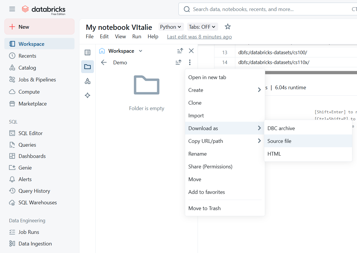
A Databricks Archive (DBC) is a proprietary file format used to export a package of notebooks and directories from a workspace. It bundles the source code, folder structure, and optionally, cell outputs into a single file. This makes it useful for manual backups or for migrating projects between different Databricks workspaces. The import and export functions are managed directly through the workspace UI.
Example Scenario
An analyst completes an initial data exploration project contained within a workspace folder named /Projects/Q3_Analysis. This folder has three notebooks and a subfolder with helper scripts. To share this entire project with a colleague who uses a different Databricks workspace, the analyst can:
- Right-click the
/Projects/Q3_Analysisfolder. - Select Export > DBC Archive.
- Send the downloaded
Q3_Analysis.dbcfile to their colleague.
The colleague can then import this single file into their own workspace, and the entire folder structure and its notebooks will be recreated instantly.
DBC vs. Git Integration
While useful, DBC archives serve a different purpose than professional source code management.
- DBC Archives: Use for simple, one-time transfers or for archiving a project with its cell outputs included.
- Databricks Repos (Git): This is the standard for production code. It provides proper version control, facilitates team collaboration through pull requests, and integrates with CI/CD pipelines for automated testing and deployment.
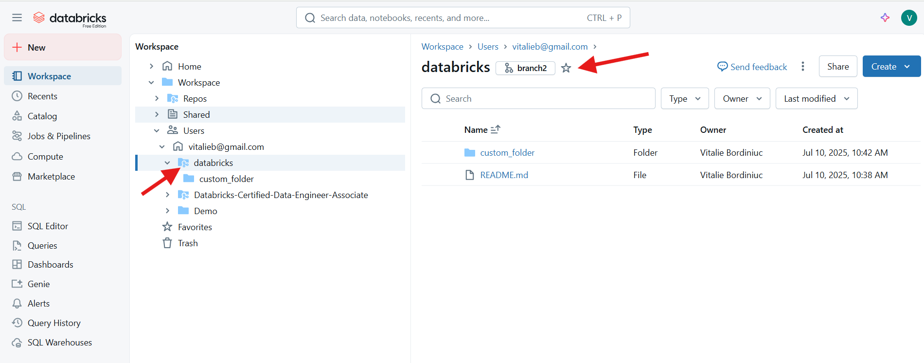
Databricks Repos (Git Integration)
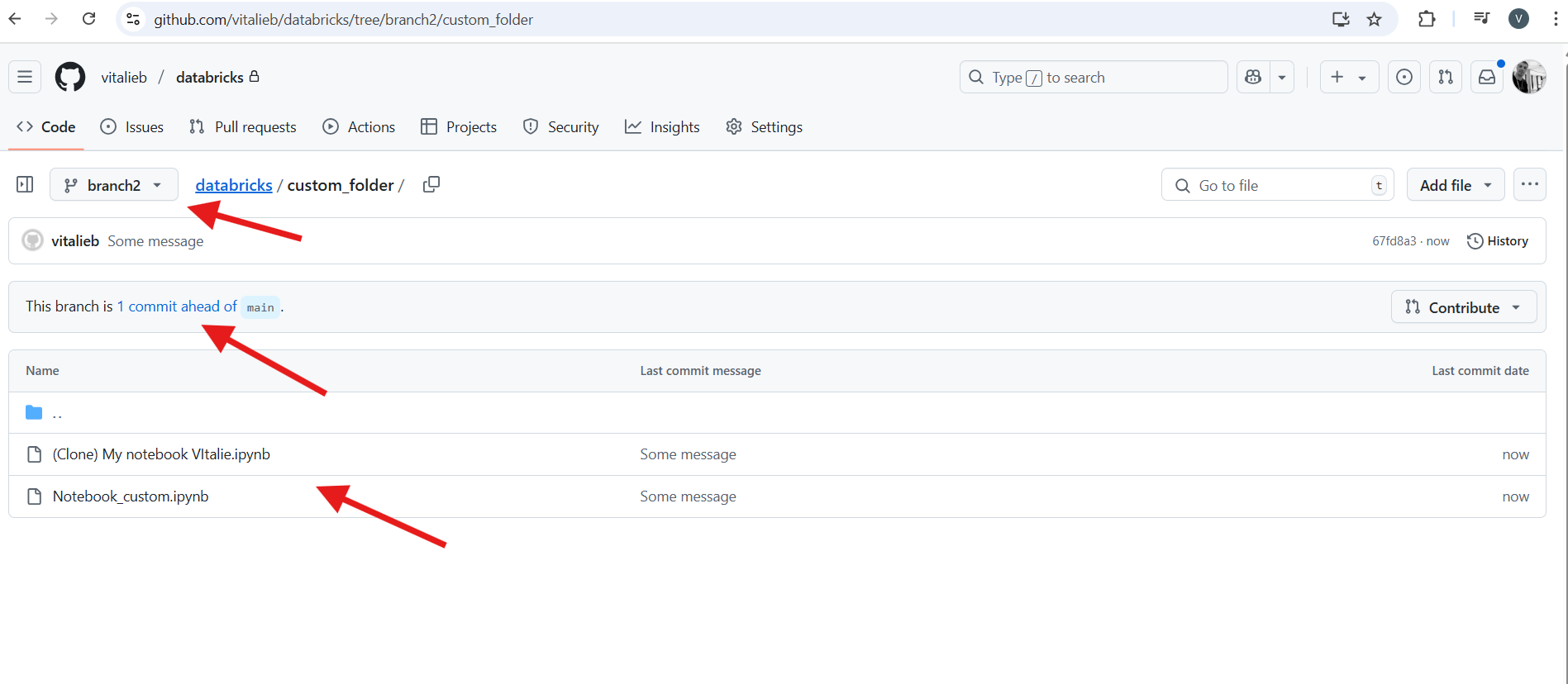
Databricks Repos syncs your workspace with remote Git repositories from providers like GitHub or GitLab. This feature lets you manage notebooks and project files with professional version control instead of as loose files in a workspace. The correct term for a folder that is synchronized with Git is a Repo.
Example Workflow
An engineer needs to add a new feature to an existing data pipeline project managed in a Databricks Repo.
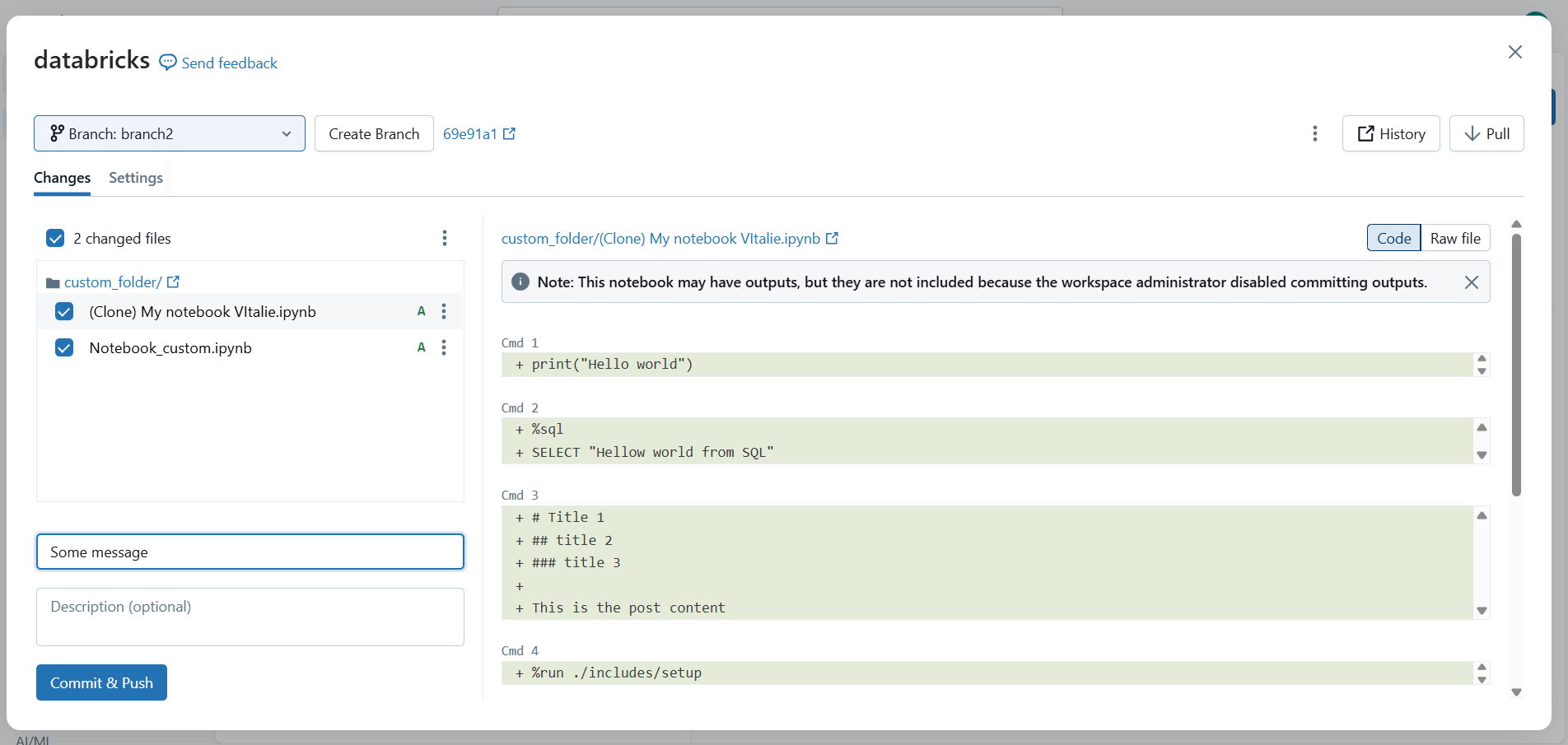
- Create a Branch: From the Databricks UI, the engineer creates a new Git branch named
feature/new-source. This creates an isolated copy of the code for development. - Develop Code: They modify the main notebook,
etl_pipeline.py, to handle the new data. They also add a helper function to a shared module,utils/helpers.py, all within the same Repo. - Commit and Push: After testing, they commit the changes with a message like “Feature: Add new API data source” and push the
feature/new-sourcebranch to the remote repository. - Create a Pull Request: In GitHub, a pull request is created. A teammate reviews the code changes. Once approved, the feature branch is merged into the
mainbranch, ensuring code quality before it becomes part of the main project.
Key Benefits
- Version Control: Every code change is tracked, allowing you to revert to previous versions if needed.
- Collaboration: Teams can work on the same project without conflict using branches and manage code quality through pull requests.
- Automation (CI/CD): Merging code into the
mainbranch can automatically trigger testing and deployment pipelines. - Code Modularity: Encourages writing reusable code in separate files (
.pyor.sql) that can be imported into notebooks.
")
